Who will hold the debt?

Today was the first day of the Fall 2026 semester. The summer went by quickly. I am happy to have the 4:15 block free on Tuesdays so I can attend the Money-Macro Workshop. Matthew Rognlie of Northwestern gave the first presentation.

His paper, The Race Between Asset Supply and Asset Demand, is joint work with Adrien Auclert, Hannes Malmberg, and Ludwig Straub. It was prepared for the 2025 Jackson Hole symposium; the working paper I read is the November 2025 version, also available as NBER Working Paper 34470.

One question ran through much of the discussion: how much does a growing desire to own wealth tell us about the demand for government debt? I kept coming back to that while reading the paper.

Two sides of an aging population

Start with the assets available for people to own. The paper adds up government debt, physical capital, and the value of claims on future profits and rents. Housing belongs here too: the structure is capital, and the land contributes to the value of rents. On the other side are the assets that households and foreign investors want to hold. The return on wealth adjusts until the two sides agree.

This takes a little getting used to. Asset supply is measured in value, relative to GDP. A fall in the required return can make an existing stream of profits more valuable, so the supply of assets can increase without anyone building another factory. The authors also allow households’ desired wealth to respond to returns. In their calibration, higher returns lead them to hold more assets, although the response is limited.

If people want to hold more wealth at a given return, asset prices rise and prospective returns fall. If more assets become available at that return, the pressure goes the other way. Both changes can leave the economy with more wealth relative to GDP. Looking at wealth alone cannot tell us which force was responsible.

Aging enters through the household side. In the wealth profiles Rognlie showed, older people hold substantially more assets than younger people, and wealth stays high well into old age. Shifting the population toward those ages increases the aggregate stock of assets people want to hold. Retirees can spend more than they earn and still own a great deal of wealth. That distinction between a flow of saving and a stock of assets is easy to lose.

The authors implement this with a shift-share calculation: hold a measured age profile of wealth fixed and change the fraction of the population at each age. They also reweight labor income by age, since everything is being expressed relative to GDP. The lifecycle model supplies conditions under which those calculations have an economic interpretation. I like being able to see what a demographic claim requires in the data.

The same older population also receives more Social Security and publicly financed healthcare. If taxes and the generosity of those programs do not adjust, the government issues more debt. Demographics therefore creates both more demand for assets and more assets to be held. How those two quantities compare is the race in the title.

What the numbers say

For 1950–2024, the paper recovers an outward shift in asset demand of about 390 percentage points of GDP, compared with about 30 on the supply side. Demand outpaced supply, pushing long-run real returns down. The demand-side explanations account for 300 points. Aging and income inequality are the largest positive contributors, followed by slower productivity growth and foreign demand. Expanded Social Security partly offsets them by reducing the need to finance retirement privately. These are shifts at a fixed return, not observed purchases or growth rates of wealth. Table 1 and Table 2 give the decomposition.

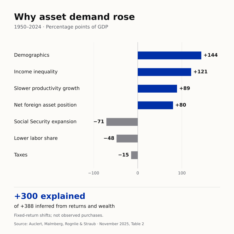
The distinction between the inferred total and the explained portion matters. With assumptions about how the two curves slope, the authors can work backward from returns and asset values to recover shifts. They then ask how much the measured drivers explain. The remaining gap is worth paying attention to. A decomposition can be informative without accounting for every movement in the data.

The small net supply shift also hides a reversal. Government debt fell from its postwar level before rising again, and the increasing value of profits and rents helped expand asset supply in the later decades. The starting date matters when reading that comparison.

Looking ahead, aging alone adds roughly 220 percentage points of GDP to asset demand by 2100 in the paper’s baseline. But unchanged benefit generosity produces a much larger fiscal burden. The authors find room for debt to reach roughly 250% of GDP at the 2024 safe rate, provided it is stabilized. Their baseline requires a permanent fiscal adjustment of around 12% of GDP. That is an annual budget change, not a one-time payment of 12% of GDP. The NBER abstract emphasizes the broader finding: even with substantial room for debt, stabilization requires an adjustment of at least 10% of GDP.

Those are conditional calculations for the end of the century. They use 2024 as their starting point, a demographic projection between the UN’s low- and medium-fertility scenarios, and assumptions about future benefits and taxes. They are not an updated forecast of the 2026 budget or a claim that borrowing can continue unchanged until 2100.

I found the two fiscal results quite compatible once I thought about them separately. There may be willing buyers for a much larger stock of debt. The government still has to bring the annual budget onto a path that stops adding debt faster than those buyers can absorb it.

Questions from the room

The strongest early exchange concerned the interest rate itself. An audience member asked whether the paper’s broad return on wealth could move differently from the safe rate relevant to monetary policy. A later question pressed on how easily investors substitute between government debt and other assets. Rognlie agreed that this was a central unresolved issue. For most of the analysis, the spread between safe and risky returns is taken as given.

That assumption has considerable weight. In the paper’s extension, where more debt erodes the government’s funding advantage, the amount of debt consistent with an unchanged safe rate falls to about 180% of GDP after allowing for older households’ greater preference for safe assets. The extension calibrates the rate response to debt more strongly than the baseline does. Figure 21 makes the sensitivity visible. Neither 180 nor 250 is a universal debt limit. Both depend on the behavior of the people holding it.

Another question went directly at the demographic evidence: was the wealth profile following people through their lives, or comparing people of different ages at one moment? It was the latter. Rognlie explained that the model handles the conversion under its assumptions, while acknowledging that differences across cohorts matter. An older homeowner and a younger renter have lived through different housing markets. Comparing their wealth today does not, by itself, tell us how much the renter will own at the same age. I would want to know how well the projection survives as new cohorts replace the ones used to construct it.

The question about fewer children made this concern more concrete. If people hold wealth partly to leave it to their children, could declining fertility change how much they want to leave behind? Rognlie said the evidence he was familiar with did not show a strong relationship between the number of children and wealth retained at death. He described this as a puzzle. It is a good question because fertility could change the wealth profile itself, in addition to changing the number of people at each age. That would give the shift-share exercise another moving part.

I also liked the questions about valuation. One participant pointed out that falling discount rates mechanically raise the value of profit claims; Rognlie confirmed that this is part of the supply curve’s slope. Later, someone asked why the US net foreign asset position had deteriorated so much when current-account deficits had been larger in an earlier period. Rognlie acknowledged the role of strong US equity performance. Foreigners’ existing claims can become more valuable without an equivalent new inflow of foreign saving. This makes the timing of the foreign-demand contribution harder to interpret.

A related objection was that interest rates are determined in a global market. The projections hold the US net foreign asset position relative to GDP fixed. Rognlie’s defense was that the US is a large part of that market and other advanced economies face similar aging pressures. That is a reasonable starting point, though a global extension could change how the extra demand is distributed across countries. More wealth held abroad does not automatically become demand for US Treasuries.

Finally, someone asked about expectations and transition dynamics. Rognlie described the approach as a sequence of long-run equilibria. The paper does phase in some effects across cohorts, but it does not solve the full path of prices and household decisions as news arrives. This seems especially relevant to fiscal policy. A credible benefit reduction announced twenty years before retirement gives someone time to respond. The same reduction arriving after retirement gives them a very different problem.

Where I would start

One question I did not hear concerns the healthcare projection. How much of the age profile of spending reflects proximity to death? If longer lives include more healthy years, carrying today’s spending at each age forward could overstate the cost. The authors flag this possibility in footnote 30. Comparing projections based on age with ones that also account for remaining life expectancy would be a useful extension.

The question I most want to pursue is whether the same fiscal news can increase desired retirement wealth while reducing the share people want to hold in government debt.

Suppose a worker becomes less confident about future retirement benefits. They may try to save more. It does not follow that they become less confident in Treasuries: a credible benefit reform could improve the government’s finances. But if the news also changes their expectations about inflation or the reliability of government commitments, their portfolio choice might change. The direction is an empirical question. I would want to measure the two responses separately.

The paper already takes a step toward this by allowing safe-asset demand to vary with age. I would extend that exercise by allowing beliefs about fiscal policy to change both total desired wealth and its allocation.

I would begin with something manageable: reconstruct wealth and portfolio profiles by age and income using the Survey of Consumer Finances, then check how stable they are across survey years. Housing, business wealth, deposits, and government securities should remain separate. For assets held through funds or pensions, I would need to examine the underlying holdings where the data allow it. A dollar in a retirement account is not necessarily a dollar financing Treasury debt.

That would still be a comparison across households. The Health and Retirement Study offers a way to follow people as they age. I would use its panel to examine changes in wealth around retirement, accounting for asset-price movements and for who remains in the sample. I would also separate households that can respond to a future benefit shortfall by saving from those that have very little room to do so. An aggregate increase in desired wealth can conceal a difficult adjustment for the people least able to make it.

To get closer to the role of beliefs, I would design a survey experiment that varies a hypothetical future benefit shortfall separately from information about the government’s financing outlook. I would ask about expected benefits, inflation, and repayment, then measure intended saving and portfolio allocations at stated returns and maturities. Keeping those features explicit would help distinguish a wish to save more from a preference for a different asset. Following up on actual contributions or account choices, where feasible, would be much more convincing than stopping at stated intentions.

There is a useful benchmark for interpreting the result. Write desired wealth as $W$ and the share allocated to government debt as $s$. Desired government-debt holdings are $sW$. For a small change,

$$d(sW) = s\,dW + W\,ds.$$

The first term captures an increase in desired wealth at an unchanged portfolio share. The second captures a change in the share itself. If that share falls enough, more desired wealth need not mean more desired government debt. This is just an accounting relationship. The research would be in learning how large the two responses are, for whom, and how quickly they occur.

Only then would I put those responses into a model with separate asset markets and explicit announcements of future fiscal changes. I would compare early, credible reform with delayed adjustment and ask how the path of financing costs changes. The survey evidence would describe one household response; any claim about national borrowing capacity would also need to account for foreign investors and financial institutions.

That feels like a worthwhile place to begin the semester. The fiscal numbers are daunting, but the questions underneath them are things we can work on: what people expect, what they save, and which promises they are willing to hold. I would be happy to spend a few more Tuesday afternoons figuring out how to measure that.